Model Building
To build a model, one needs to understand the physical properties of the obersved process. Many processes can be described using differential equations. When solved, these equations can describe a linear or non-linear model.
TL;DR: How to Build Models
Modeling involves the description of some observable data using a mathematical equation that describes the underlying physical properties of the experiment.
Our process is as such:
-
We need to identify a general, mathematical model that can represent the observed data. The parameters of the model describe the specifics of the data.
-
We need to determine the values of the parameters in the model that best fit our data. This is accomplished by a fitting algorithm that minimizes the differences between the data and the model. Generally, an initial estimate is required that is then improved.
-
We need to estimate the error in the parameters we determined in the fitting process to obtain the confidence intervals
EXAMPLE: Radioactive Decay Model Building
Hypothesis: The rate of decay is proportional to the number of nuclei present
Mathematical Model:
Solve:
MODELS FOR REACTING SYSTEMS:
The magnitude of the measureable off-rate depends on the rotor speed and sedimentation coefficient.
For faster rotor speeds, higher molecular weight and globular shape will favour the measurement of faster rate constants.
Data Fitting
Any observable process that influences the measurement needs to be acccounted for in order for models to yeld any meaningful result. The object is then to minimize the residuals between the model and the data.
Iverse preoblem: extracting parameters from a simulated solution by fitting the model to experimental data.
A non-parametric fit is used to smooth data for display, where the instrinsic model is of little intrest, and hence the parameters are not needed.
Method of Least-Squares
When useing the Method of Least Squares, we make the following assumptions:
-
The model is a truthful representation of reality.
-
All error is ssociated with a dependent variable.
-
All experimental noise is considered to be of Gaussian distribution.
The minimum in the differences occur when the derivative of our objective function with respect to the parameters is zero, so we need to differentiate it with respect to the parameters of interest, a and b. This will lead to a system of linear equations.
Any observable process that influences the measurement needs to be accounted for in order for the model to yield meaningful results. Our objective is then to minimize the residuals between the model and the data:
Extracting parameters from the simulated solution by fitting the model to experimetal data is called an \(\bf{\text{Inverse Problem}}\).
LEAST-SQUARES EQUATION FOR STRAIGHT LINES: The equation for a straight line is a linear equation: y = mx +b. Remember our least squares equation above; for a straight line, it changes to:
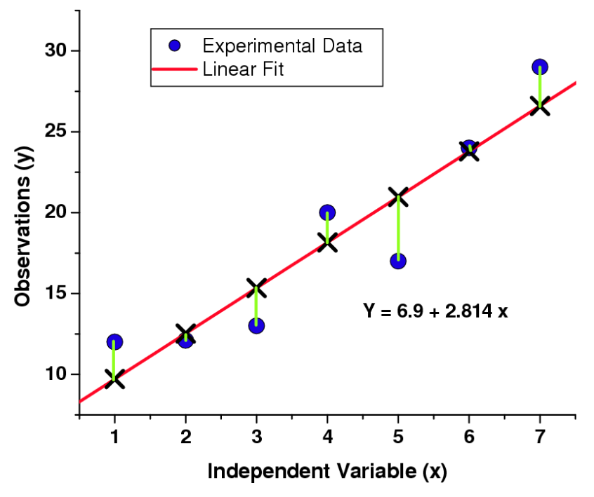
The distances from the experimental data and the linear fit are measured to be perpendicular to the data (see figure), and the objective of this method is to find the equation of a straight line that minimizes the distance between the data and the fit.

SOLVING THE LEAST SQUARES EQUATION (LINEAR LINE): The minimum in the differences between our data and our fit occurs when the derivative of our function (with respect to the parameters) is zero. Therefore, we must take our least squares equation and differentiate it:
With respect to parameter \(a\):
With respect to parameter \(b\):
This will lead to a system of linear equations:
When in matrix form, this system of equations can be solved by using Cramer's rule, such that:
Linear Models
As discussed above, we know that the equation for a linear equation is \(y = a + bx\), and we know that the equation is linear in the coefficients that are fitted. In fact, the equation doesnt have to be that of a straight line to be considered linear. Rather, we can express it with a polynomial:
Then, as long as the coefficients are linear, the equation will be considered a linear fitting equation. It does not matter how wildly non-linear the terms of the independent variable are. For example, our variables can be exponentials, or trignometric functions (all of which are not linear):
with \(X_{n}\) being any non-linear term. That being said, sometimes we may want to constrain the value of a paramater. For example, suppose we do not want the amplitude of an exponential term to turn negative during the fitting process. We can prevent this by fitting the log of a number, such that the fitted value will never be negative.
EXAMPLE: Linearization
Linearization of a Non-Linear Equation
Suppose we have an exponential equation of the form:
To linearize it, we take the natural logarithm on both side.
Non-Linear Regression
What is the importance of an equation being linear or non-linear? It turns out that non-linear functions require fitting using iterative approaches, while linear functions can be fitted using a single interation. Consider the Jacobian matrix for non-linear systems:
We are hoping to iteratively improve the parameter estimates by following along the gradient of the error functino in the direction of maximum imporovement. This requires knowledge of the partial derivatives of each parameters at each point in the experiment. Let us therefore take:
where \(\bf{J}\) is the Jacobian matrix, shown above, \(g\) is the current parameter estimate, \(a\) is the adjustment made to the parameter estimate in the current iternation, and \(\Delta y\) is the difference between the experimental data and the model. To solve for the value of \(a\):
Once here, we have two options. Option 1:
Option 2 is when \(\bf{J}^{T}\bf{J}\) is positive, so that we can use the Cholesky decomposition (\(\bf{J}^{T}\bf{J} = \bf{LL}^{T}\)).
We then iterate until the function converges.
EXAMPLE: Appropriateness of Fitting Approaches
For each of the following situations, what is the fitting approach. Is it non-parametric, gradient descent, grid method, or stochastic? Is it linear or non-linear in its fitting parameters? If the appraoch is non-parametric, propose a function for it.
A. Smoothing a set of noisy data with a recognizable wave pattern
B. Fitting parameters \(a\) and \(b\) from function:
C. Fitting paramaters \(a_{i}\) from function:
D. Fitting paramaters \(a_{j}\) from function:
E. Fitting parameters \(a, b\), and \(c\) from function:
F: Fitting parameters \(a_{1}\) to \(a_{8}\):
Experimental Uncertainties, Error Surfaces, and Fit Quality

EXPERIMENTAL UNCERTAINTIES: The uncertainty of an measurement can be determined by repeating the expriment several times. Each time, a slightly different value is obtained for the experimental observation. If we assume a Gaussian distribution of errors in the measurement, we can determine the standard deviation, \(\sigma\), of the distribution of measured parametes. Then we can use \(\sigma\) to set the error bars on the measurement and to scale the contribution of a datapoint to the sum of residuals.
To calculate the standard deviataion, use the following equation:
where \(\bar x\) is the average of all measurements.

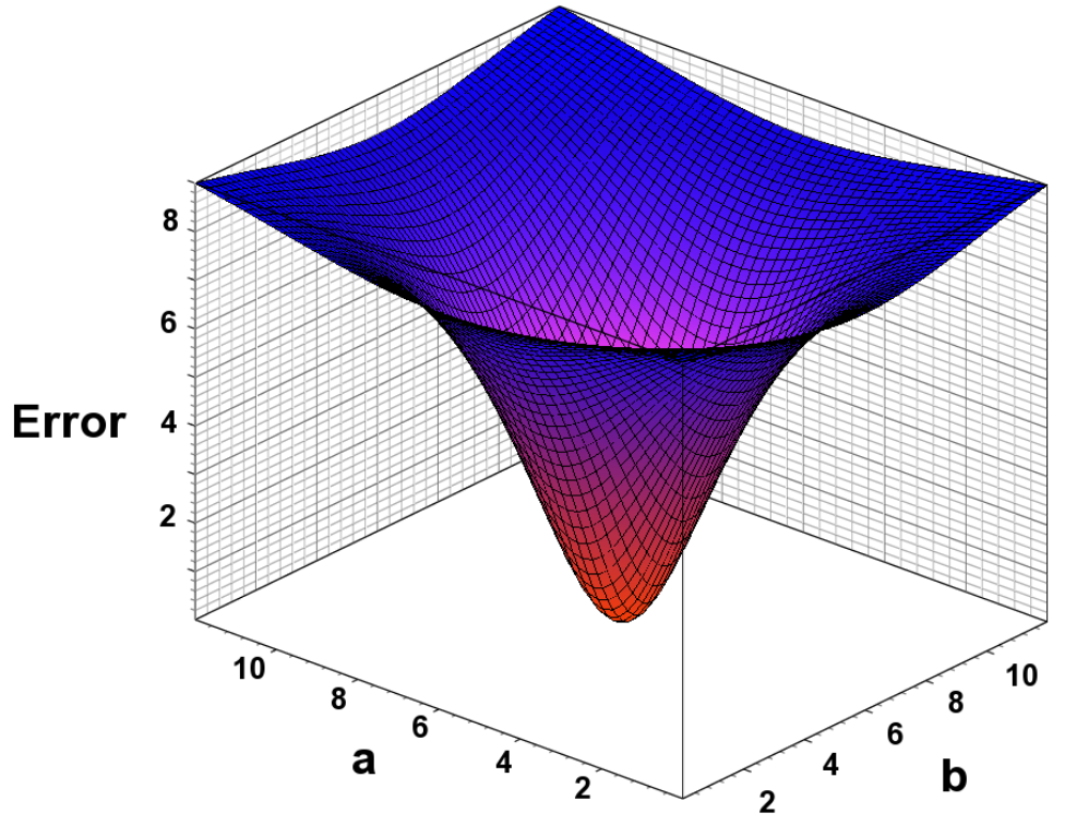
ERROR SURFACES: Each parameter combination a, b results in a unique error when fitted to the experimental data. The optimal solution occurs where the error is the smallest. Ideally, the error surface is continuously differentiable.
GOODNESS OF FIT: The quality of the fit is determined by the randomness of the residuals, and the root mean square deviatio (RMSD). The randomness of the residuals can be measured by determining the runs. Runs (R) are the number of consecutive positive (p) or negative (n) residuals from the mean.
where \(R_{T}\) is the measure of randomness, and:
Optimization Methods
For linear fits, our options for optimizing methods include straight line fits, generalized inear least squares, non-negative constrained least squares, multi-dimensional spectrum analyses, and non-parametric fits. Examples of non-parametric fits are B-splines and polynomial smoothing.
For non-linear optimizatin using gradient descent methods for functions of type, \(y = F(a_{i},x_{i})\), we can use Levenberg-Marquardt, Gauss-Newton, Quasi-Netwon, conjugate gradients, tangent approximation, or neural networks. A problem with non-linear least squares optimization is that for multi-component systems, the algorithm gets easily stuck in local minima and the solution will depend on the starting points. This problem gets worse when there are more parameters.
TL;DR: Optimization Methods
These will be discussed in more detail on their own pages.
2DSA: Provides degenerate, linear fits to experimental data over a finite domain, identifying regions with signal in the mass/shape domain, used to remove systematic noise contributions
GA: provides parsimonious regularization of 2DSA spectrums, statisfies Occam's razor. Also used for fitting of discrete, non-linear models (reversible associations, non-ideality, co-sedimenting solutes)
MC: used to measure the effect of noise on fitted parameters, yields parameter distribution statistics
PCSA: used to regularize 2DSA, enforces a unique mapping of one molar mass/sedimentation coefficient per frictional ratio.
There are also stochastic (Monte Carlo, simulated annealing, random walk, and genetic algorithms) and deterministic fitting methods.
For comparrison:
STOCHASTIC:
-
large search space possible
-
generally slow converging
-
excellent convergence properties with enough time
-
computer-intensive
-
suitiable for many parameters
-
good for ill-conditioned error surfaces
-
derivates not needed
DETERMINISTIC:
-
small search space
-
suitable for a few parameters only
-
well-conditioned error surface
-
very fast convergence
-
requires derivatives